This blog post is the first part of a series of 3 articles related to the PipeWire project and its usage in embedded Linux systems.

Introduction

PipeWire is a graph-based processing engine, that focuses on handling multimedia data (audio, video and MIDI mainly).

It has gained steam early on by allowing screen sharing on Wayland desktops, which for security reasons, does not allow an application to access any framebuffer that does not concern it. The PipeWire daemon was run with sufficient privileges to access screen data; giving access through a D-Bus service to requesting applications, with file-descriptor passing for the actual video transfer. It was as such bundled in the Fedora distribution, version 27.

Later on, the idea was to expand this to also allow handling audio streams in the processing graph. Big progress has been done by Wim Taymans on this front, and PipeWire is now the default sound server of the desktop Fedora distribution, since version 34.

The project is currently in active development. It happens in the open, lead by Wim Taymans. The API and ABI can both be considered stable, even though version 1.0 has not been released yet. The changelog exposes very few breaking changes (two years without one) and many bug fixes. It is developed in C, using a Meson and Ninja based build system. It has very few unconditional runtime dependencies, but we’ll go through those during our first install.

Throughout this series of blog articles, our goal will be to discover PipeWire and the possiblities it provides, focusing upon audio usage on embedded platforms. A detailed theoretical overview at the start will allow us to follow up with a hands-on approach. Starting with a minimal Buildroot setup on a Microchip SAMA5D3 Xplained board, we will create then our own custom PipeWire source node. We will then study how dynamic, low-latency routing can be done. We’ll end with experiments regarding audio-over-ethernet.

A note: we will start with many theoretical aspects, that are useful to get a good mental model of the way PipeWire works and how it can be used to implement any wanted behavior. This introduction might therefore get a little exhaustive at times, and it could be a good approach to skip even if a concept isn’t fully grasped, to come back later during hands-ons when details on a specific subject is required.

Sky-high overview

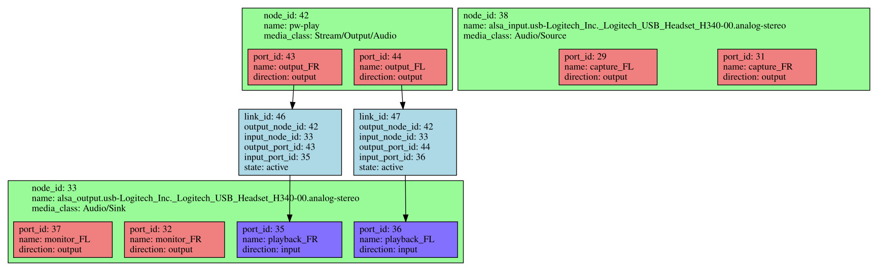
A PipeWire graph is composed of nodes. Each node takes an arbitrary number of inputs called ports, does some processing over this multimedia data, and sends data out of its output ports. The edges in the graph are here called links. They are capable of connecting an output port to an input port.

Nodes can have an arbitrary number of ports. A node with only output ports is often called a source, and a sink is a node that only possesses input ports. For example, a stereo ALSA PCM playback device can be seen as a sink with two input ports: front-left and front-right.

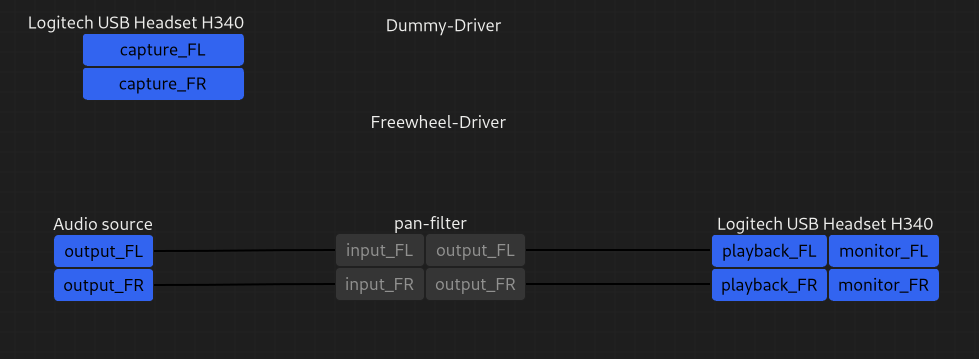
Here is a visual representation of a PipeWire graph instance, provided by the Helvum GTK patchbay:

Visual attributes are used in Helvum to describe the state of nodes, ports and links:

• Node names are in white, with their ports being underneath the names. Input ports are on the left while output ports are on the right.
• “Dummy-Driver” and “Freewheel-Driver” nodes have no ports. Those two are particular sinks (with dynamic input ports, that appear when we connect a node to them) used in specific conditions by PipeWire.
• Red means MIDI, yellow means video and blue means audio.
• Links are solid when active (data is “passing-through” them) and dashed when in a paused state.

Note: if your Linux desktop is running PipeWire, trying installing Helvum to graphically monitor and edit your multimedia graph! It is currently packaged on Fedora, Arch Linux, Flathub, crates.io and others.

Design choices

There are a few noticeable design choices that explain why PipeWire is being adopted for desktop and embedded Linux use cases.

Session and policy management

One first design choice was to avoid tackling any management logic directly inside PipeWire; context-dependent behaviour such as monitoring for new ALSA devices, and configuring them so that they appear as nodes, or automatically connecting nodes using links is not handled. It rather provides an API that allows spawning and controlling those graph objects. This API is then relied upon by client processes to control the graph structure, without having to worry about the graph execution process.

A pattern that is often used and is recommended is to have a single client be a daemon that deals with the whole session and policy management. Two implementations are known as of today:

• pipewire-media-session, which was the first implementation of a session manager. It is now called an example and used mainly in debugging scenarios.
• WirePlumber, which takes a modular approach: it provides another, higher-level API compared to the PipeWire one, and runs Lua scripts that implement the management logic using the said API. In particular, this session manager gets used in Fedora since version 35. It ships with default scripts and configuration that handle linking policies as well as monitoring and automatic spawning of ALSA, bluez, libcamera and v4l2 devices. The API is available from any process, not only from WirePlumber’s Lua scripts.

Individual node execution

As described above, the PipeWire daemon is responsible for handling the proper processing of the graph (executing nodes in the right order at the right time and forwarding data as described by links) and exposing an API to allow authorized clients to control the graph. Another key point of PipeWire’s design is that the node processing can be done in any Linux process. This has a few implications:

• The PipeWire daemon is capable of doing some node processing. This can be useful to expose a statically-configured ALSA device to the graph for example.
• Any authorized process can create a PipeWire node and be responsible for the processing involved (getting some data from input ports and generating data for output ports). A process that wants to play stereo audio from a file could create a node with two output ports.
• A process can create multiple PipeWire nodes. That allows one to create more complex applications; a browser would for example be able to create a node per tab that requests the ability to play audio, letting the session manager handle the routing: this allows the user to route different tab sources to different sinks. Another example would be an application that requires many inputs.

API and backward compatibility

As we will see later on, PipeWire introduces a new API that allows one to read and write to the graph’s overall state. In particular, it allows one to implement a source and/or sink node that will be handling audio samples (or other multimedia data).

One key point for PipeWire’s quick adoption is a focus on providing a shim layer to currently-widespread audio API in the Linux environment. That is:

• • It can obviously expose ALSA sinks or sources inside the graph. This is at the heart of what makes PipeWire useful: it can interact with local audio hardware. It uses alsa-lib as any other ALSA client. PipeWire is also capable of creating virtual ALSA sinks or sources, to interface with applications that rely solely upon the alsa-lib API.
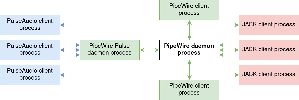
  • It can implement the PulseAudio API in place of PulseAudio itself. This simply requires starting a second PipeWire daemon, with a specific pulse configuration. Each PulseAudio sink/source will appear in the graph, as if native. PulseAudio is the main API used by Linux desktop users and this feature allows PipeWire to be used as a daily-driver while supporting all standard applications. An anecdote: relying on the PulseAudio API is still recommended for simple audio applications, for its more widespread and simpler API.
  • It also implements the JACK Audio Connection Kit (or JACK); this API has been in use by the pro-audio audience and targets low-latency for audio and MIDI connections between applications. This requires calling JACK-based applications using pw-jack COMMAND, which does the following according to its manual page:

pw-jack modifies the LD_LIBRARY_PATH environment variable so that applications will load PipeWire’s reimplementation of the JACK client libraries instead of JACK’s own libraries. This results in JACK clients being redirected to PipeWire.

About compatibility with Linux audio standards, the PipeWire FAQ has an interesting answer to the expected question whenever something new appears: why another audio standard, Linux already has 13 of them? For exhaustiveness, here is a quick rundown of the answer: it describes how Linux has one kernel audio subsystem (ALSA) and only two userspace audio servers: PulseAudio and JACK. Others are either frameworks relying on various audio backends, dead projects or wrappers around audio backends. PipeWire’s goal, on the audio side, is to provide an alternative to both PulseAudio and JACK.

Real-time execution: push or pull?

In the simple case of a producer and a consumer of data, two execution models are in theory possible:

• Push, where the producer generates data when it can into a shared buffer, from which the consumer reads. This is often associated with blocking writes to signal the producer when the buffer is full.
• Pull, where the producer gets signaled when data is needed for the consumer, at which point the producer should generate data as fast as possible into the given shared buffer.

In a real-time case scenario, latency is optimal when the data quantity in the shared buffer is minimised: when the producer adds data to the buffer, all the data already present in the buffer needs to be consumed before the new data gets processed as well. As such, the pull method allows the system to monitor the shared buffer state and signal the producer before the shared buffer gets empty; this guarantees data that is as up-to-date as possible as it was generated as late as possible.

That was for a generic overview of pushed versus pulled communication models. PipeWire adopts the pull model as it has low latencies as a goal. Some notes:

• The structure is more complex compared to a single producer and single consumer architecture, as there can be many more producers and consumers, possibly with nodes depending on multiple other nodes.
• The PipeWire daemon handles the signaling of nodes. Those get woken up, fill a shared memory buffer and pass it onto its target nodes; those are the nodes that take its output as an input (as described by link objects).
• The concept of driver nodes is introduced; other nodes are called followers. For each component (subgraph of the whole PipeWire graph), one node is the driver and is responsible for timing information. It is the one that signals PipeWire when a new execution cycle is required. For the simple case of an audio source node (the producer) and an ALSA sink node (the consumer), the ALSA sink will send data to the hardware according to a timer, signaling PipeWire to start a new cycle when it has no more data to send: it pulls data from the graph by telling it that it needs more.

Note: in this simple example, the buffer size provided to ALSA by PipeWire determines the time we have to generate new data. If we fail to execute the entire graph in time before the timer, the ALSA sink node will have no data and this will lead to an underrun.

Implementation overview

This introduction and the big design decisions naturally lead us to have a look at the actual implementation concepts. Here are the questions we will try to answer:

• How is the graph state represented?
• How can a client process get access to the graph state and make changes?
• How is IPC communication handled?

Graph state representation: objects, objects everywhere

As said previously, PipeWire’s goal is to maintain, execute and expose a graph-structured multimedia execution engine. The graph state is maintained by the PipeWire daemon, which runs the core object. A fundamental principle is the concept of an object. Clients communicate with the core using IPC, and can create objects of various types, which can then be exported. Exporting an object means telling the core and its registry about it, so that the object becomes a part of the graph state.

Every object have at least the following: a unique integer identifier, some permissions flags for various operations, an object type, string key-value pairs of properties, methods and event types.

Object types

There is a fixed type list, so let’s go through the main existing types to understand the overall structure better:

• The core is the heart of the PipeWire daemon. There can only be one core per graph instance and it has the identifier zero. It maintains the registry, which has the list of exported objects.
• A client object is the representation of an open connection with a client process, from within the daemon process.
• A module is a shared object that is used to add functionality to a PipeWire client. It has an initialisation function that gets called when the module gets loaded. Modules can be loaded in the core process or in any client process. Clients do not export to the registry the modules they load. We’ll see examples of modules and how to load them later on.
• A node is a producer and/or consumer of data; its main characteristic is to have input and output port objects, which can be connected using link objects to create the graph structure.
• A port belongs to a node and represents an input or output of data. As such, it has a direction, a data format and can have a channel position if it is audio data that is being transferred.
• A link object connects two ports of opposite direction together; it describes a graph edge.
• A device is a handle representing an underlying API, which is then used to create nodes or other devices. Examples of devices are ALSA PCM cards or V4L2 devices. A device has a profile, which allows one to configure them.
• A factory is an object whose sole capability is to create other objects. Once a factory is created, it can only emit the type of object it declared. Those are most often delivered as a module: the module creates the factory and stays alive to keep it accessible for clients.
• A session object is supposed to represent the session manager, and allow it to expose APIs through the PipeWire communication methods. It is not currently used by WirePlumber but this is planned.
• An endpoint is the concept of a (possibly empty) grouping of nodes. Associated with endpoint streams and links, they can represent a higher-level graph that is handled by the session manager. Those would allow modeling complex behaviors such as mutually-exclusive sinks (think laptop speakers and line-out port) or nodes to which PipeWire cannot send audio streams, such as analog peripherals for which the streams do not go through the CPU. Those peripherals would therefore appear in the graph, be controlled with the same API (routing using links, setting volume, muting, etc.) but the processing would be done outside PipeWire’s reach. See PipeWire’s documentation for more information on the potential of those advanced features.

Permissions

The session and policy manager (most often WirePlumber) is also responsible for defining the list of permissions each client has. Each permission entry is an object ID and four flags. A special PW_ID_ANY ID means that those permissions are the default, to be used if a specific object is not described by any other permission. Here are the four flags:

• Read: the object can be seen and events can be received;
• Write: the object can be modified, usually through methods (which requires the execute flag);
• eXecute: methods can be called;
• Metadata: metadata can be set on the object.

This isn’t well leveraged upon yet, as all clients get default permissions of rwxm: read, write, execute, metadata.

Properties

All objects also have properties attributed to them, which is a list of string key-value pairs. Those are abitrary and various keys are expected for various object types. An example link object has the following properties (as reported by pw-cli info LINK_ID):

# Link ID
object.id = "95"

# Source port
link.output.node = "91"
link.output.port = "93"

# Destination port
link.input.node = "80"
link.input.port = "86"

# Client that created the link
client.id = "32"

# Factory that was called to create the link
factory.id = "20"

# Serial identifier: an incremental identifier that guarantees no
# duplicate across a single instance. That exists because standard
# IDs get reused to keep them user-friendly.
object.serial = "677"

Parameters

Some object types also have parameters (often abbreviated as params), which is a fixed-length list of parameters that the object possesses, specific to the object type. Currently, nodes, ports, devices, sessions, endpoints and endpoint streams have those. Those params have flags that define if they can be read and/or written, allowing things like constant parameters defined at the object creation.

Parameters are the key that allow WirePlumber to negotiate data formats and port configuration with nodes: hardware that supports multiple sample rates? channel count and positions? sample format? enable monitor ports? etc. Nodes expose enumerations of what they are capable of, and the session manager writes the format/configuration it chose.

Methods & events

An object’s implementation is defined by its list of methods. Each object type has a list of methods that it needs to implement. One note-worthy method is process, that can be found on nodes. It is the one that eats up data from input ports and provides data for each output port.

Every object implement at least the add_listener method, that allows any client to register event listeners. Events are used through the PipeWire API to expose information about an object that might change over time (the state of a node for example).

Exposing the graph to clients: libpipewire and its configuration

Once an object is created in a process, it can be exported to the core’s registry so that it becomes a part of the graph. Once exported, an object is exposed and can be accessed by other clients; this leads us into this new section: how clients can get access and interact with the graph.

The easiest way to interact with a PipeWire instance is to rely upon the libpipewire shared object library. It is a C library that allows one to connect to the core. The connection steps are as follows:

1. Initialise the library using pw_init, whose main goal is to setup logging.
2. Create an event-loop instance, of which PipeWire provides multiple implementations. The library will later plug into this event-loop to register event listeners when requested.
3. Create a PipeWire context instance using pw_context_new. The context will handle the communication process with PipeWire, adding what it needs to the event-loop. It will also find and parse a configuration file from the filesystem.
4. Connect the context to the core daemon using pw_context_connect. This does two things: it initialises the communication method and it returns a proxy to the core object.

Proxies

A proxy is an important concept. It gives the client a handle to interact with a PipeWire object which is located elsewhere but which has been registered in the core’s registry. This allows one to get information about this specific object, modify it and register event listeners.

Event listeners are therefore callbacks that clients can register on proxy objects using pw_*_add_listener, which takes a struct pw_*_events defining a list of function pointers; the star should be replaced by the object type. The libpipewire library will tell the remote object about this new listener, so that it notifies the client when a new event occurs.

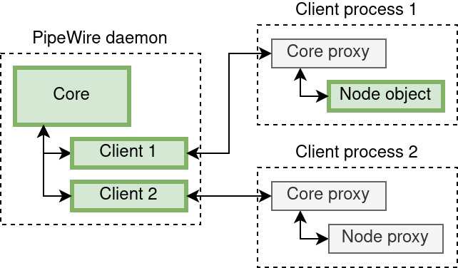
We’ll take an example to describe the concept of proxies:

In this schema, green blocks are objects (the core, clients and a node) and grey ones are proxies. Dotted blocks represent processes. Here is what would happen, in order, assuming client process 2 wants to get the the state of a node that lives in client process 1:

1. Client process 2 creates a connection with the core, that means:
   • On the daemon side, a client object is created and exported to the registry;
   • On the client side, a proxy to the core object is acquired, which represents the connection with the core.
2. It then uses the proxy to core and the pw_core_get_registry function to get a handle on the registry.
3. It registers an event listener on the registry’s global event, by passing a struct pw_registry_events to pw_registry_add_listener. That event listener will get called once for each object exported to the registry.
4. The global event handler will therefore get called once with the node as argument. When this happens, a proxy to the node can be obtained using pw_registry_bind and the info event can be listened upon using pw_node_add_listener on the node proxy with a struct pw_client_events containing the list of function pointers used as event handlers.
5. The info event handler will therefore be called once with a struct pw_node_info argument, that contains the node’s state. It will then be called each time the state changes.

The same thing is done in tutorial6.c to print every clients’ information.

Context configuration

When a PipeWire context is created using pw_context_new, we mentioned that it finds and parses a configuration file from the filesystem. To find a configuration file, PipeWire requires its name. It then searches for this file in following locations, $sysconfdir and $datadir being PipeWire build variables:

1. Firstly, it checks in $XDG_CONFIG_HOME/pipewire/ (most probably ~/.config/pipewire/);
2. Then, it looks in $sysconfdir/pipewire/ (most probably /etc/pipewire/);
3. As a last resort, it tries $datadir/pipewire/ (most probably /usr/share/pipewire/).

PipeWire ships with default configuration files, which are often put in the $datadir/pipewire/ path by distributions, meaning those get used as long as they have not been overriden by custom global configuration files (in $sysconfdir/pipewire/) or personal configuration files (in $XDG_CONFIG_HOME/pipewire/). Those are namely:

• pipewire.conf, the daemon’s configuration file;
• pipewire-pulse.conf, for the daemon process that implements the PulseAudio API;
• client.conf, for processes that want to communicate using the PipeWire API;
• client-rt.conf, for processes that want to implement node processing, RT meaning realtime;
• jack.conf, used by the PipeWire implementation of the JACK shared object library;
• minimal.conf, meant as an example for those that want to run PipeWire without a session manager (static configuration of an ALSA device, nodes and links).

The default configuration name used by a context is client.conf. This can be overriden either through the PIPEWIRE_CONFIG_NAME environment variable or through the PW_KEY_CONFIG_NAME property, given as an argument to pw_context_new. The search path can also be modified using the PIPEWIRE_CONFIG_PREFIX environment variable.

Make sure to go through one of them to get familiar with them! The format is described as a “relaxed JSON variant”, where strings do not need to be quoted, the key-value separator is an equal symbol, commas are unnecessary and comments are allowed starting with an hash mark. Here are the sections that can be found in a configuration file:

• context.properties, that configures the context (log level, memory locking, D-Bus support, etc.). It is also used extensively by pipewire.conf (the daemon’s configuration) to configure the graph default and allowed settings.
• context.spa-libs defines the shared object library that should be used when a SPA factory is asked for. The default values are best to be kept alone.
• context.modules lists the PipeWire modules that should be loaded. Each entry has an associated comment that explains clearly what each modules does. As an example, the difference between client.conf and client-rt.conf is the loading of libpipewire-module-rt that turns on real-time priorities for the process and its threads.
• context.objects allows one to statically create objects by providing a factory name associated with arguments. This is what is used by the daemon’s pipewire.conf to create the dummy node, or by minimal.conf to statically create an ALSA device and node as well as a static node.
• context.exec lists programs that will be executed as childs of the process (using fork(2) followed by execvp(3)). This was primarily used to start the session manager; it is however recommended to handle its boot separately, using your init system of choice.
• filter.properties and stream.properties are used in client.conf and client-rt.conf to configure node implementations. Filters and streams are the two abstractions that can be used to implement custom nodes, which we will talk in detail in a later article.

Inter-Process Communication (IPC)

Being a project that handles multimedia data, transfers it in-between processes and aims for low-latency, the inter-process communication it uses is at the heart of its implementation.

Event loop

The event-loop described previously is the scheduling mechanism for every PipeWire process (the daemon and every PipeWire client process, including WirePlumber, pipewire-pulse and others). This loop is an abstraction layer over the epoll(7) facility. The concept is rather simple: it allows one to monitor multiple file descriptors with a single blocking call, that will return once one file descriptor is available for an operation.

The main entry point to this event loop is pw_loop_add_source or its wrapper pw_loop_add_io, which adds a new file descriptor to be listened for and a callback to take action once an operation is possible. In addition to the loop instance, the file descriptor and the callback, it takes the following arguments:

• A mask describing the operations for which we should be waken up: read(2) is possible (SPA_IO_IN), write(2) is possible (SPA_IO_OUT), an error occured (SPA_IO_ERR) and a hang-up occured (SPA_IO_HUP);
• A boolean describing whether the file descriptor should be closed automatically at the end of not;
• A void pointer given to the callback; this is often called user data which means we can avoid static global variables.

Note: this event loop implementation is not reserved to PipeWire-related processing; it can be used as a main event loop in your processes.

That leads us to the other synchronisation and communication primitives used, which are all file-descriptor-based for integration with the event loop.

File-descriptor-based IPC

eventfd(2) is used as the main wake-up method when that is required, such as with node objects that must run their process method. signalfd(2) is used to register signal callbacks in the event-loop.

epoll(7), eventfd(2) and signalfd(2) being Linux-specific, it should be noted that there is an abstraction layer that allows one to use other primitives for implementations. Currently, Xenomai primitives are supported through this layer.

The main communication protocol is based upon a local streaming socket(2): socket(PF_LOCAL, SOCK_STREAM | SOCK_CLOEXEC | SOCK_NONBLOCK, 0). The encoding scheme used is called Plain Object Data (POD) and is a rather simple format; a POD has a 32-bits size, a 32-bits type followed by the content. There are basic types (none, bool, int, string, bytes, etc.) and container types (array, struct, object and sequence). In top of this encoding scheme is provided the Simple Plugin API (SPA) which implements a sort of Remote Procedure Call (RPC). See this PipeWire under the hood blog article that has a detailed section on POD, SPA and example usage of the provided APIs.

D-Bus

PipeWire and WirePlumber also optionally depend on the higher-level D-Bus communication protocol for specific features:

• Flatpaks are desktop sandboxed applications, that rely on portal (a process that exposes D-Bus interfaces) to access system-wide features such as printing and audio. In our case, libpipewire-module-portal allows the portal process to handle permission management relative to audio for Flatpak applications. See module-portal.c and xdg-desktop-portal for more information.
• WirePlumber, through its module-reserve-device, supports the org.freedesktop.ReserveDevice1 D-Bus interface. It allows one to reserve an audio device for exclusive use. See the quick and to-the-point specification about the interface for more information.
• D-Bus support is required if Bluetooth is wanted, to allow communication with the BlueZ process. See the SPA bluez5 plugin.

Conclusion

Now that the overall concepts as well as design and implementation choices have been covered, it is time for some hands-on! We will carry on with a bare install based upon a Linux kernel and a Buildroot-built root filesystem image. Our goal will be to output sound to an USB ALSA PCM sink, from an audio file.

Do not hesitate to come back to this article later on, that might help you clear-up some blurry concepts if needed!