As part of a recent project involving advanced sound cards, Bootlin engineer Miquèl Raynal had to find a way to automate audio hardware loopback testing. In hand, he had a PCI audio device with many external interfaces, each of them featuring an XLR connector. The connectors were wired to analog and digital inputs and outputs. In a regular sound-engineers based company, playing back heavy music through amplifiers and loud speakers is probably the norm, but in order to prevent his colleagues ears from bleeding during his ALSA/DMA debug sessions, he decided to anticipate all human issues and save himself from any whining coming from his nearby colleagues.

The solution: wiring the outputs into the inputs, record what is being played back and compare. The approach has at least one drawback: in case of an issue, because playback and capture are serially chained, both sides could be the problem, without being able to tell which one is at fault. At least, it helps knowing if something is wrong and allows to automate the checking.

Another goal of the work was to write an ALSA configuration file as explained in this blog post to leverage all the possibilities offered by ALSA-lib to split or merge several channels together and offer virtual PCMs to the user. In order to validate the correct behavior of this configuration, we need to verify how audio streams would be distributed across the different channels.

Most of the existing tools we had available turned out being either too complex or not fitted for our particular needs. It therefore appeared necessary to write a set of simple tools to generate and analyze sound automatically, based on the common ALSA tools: aplay and arecord.

The background idea was to create two tools. A first one generating a *.wav file, with a controlled number of channels, each of them filled with a known number of sine-waves generated at expected frequencies, spread all around a usable range. The file generated by this tool would be played back by the sound device. The second tool would receive as input a recorded *.wav file, extract each channel, perform its analysis, extract the main frequencies out of each channel and eventually compare them with the expected ones. A similar idea had already been done to test display interfaces in the igt-gpu-tools by another Bootlin engineer, Paul Kocialdowski, and the work presented below was highly inspired from this original tool (see our previous blog posts here and here).

Sound generation

The wave

The most trivial type of sound file is a pure sine-wave. Despite being highly unpleasant for the human ear, sine-waves are beautiful mathematical tools, easy to generate and easy to extract.

Mathematically speaking, a sine-wave w is defined by:
w(t) = sin(2*PI*f*t + k), with:

• f, the wave frequency
• t, the moment in time
• k, the phase of the signal

In our tools we can simply ignore the phase which would have no impact, thus k = 0.

The above formula works in the case of continuous waves but we have to work with discrete digital values. Translating this into a real world case, we can use:
t = s / Fs, with:

• s, the sample
• Fs, the sampling frequency, in other words the number of samples in one second

Fortunately, because sin(x) == sin(2PI + x), we do not need to care about the upper bounds, the signal will remain periodic anyway.

An array of samples containing such output would be analyzed like an almost perfect sine-wave. If several frequencies must be carried in the same audio buffer, the different sine-waves thus produced can be summed. The audio intensity can also be normalized by dividing the final value by the number of channels, that is kind of optional but looks nicer.

The audio content

We want to generate audio files with several channels. In order to be able to distinguish the frequencies on each channel, requesting different frequencies on each of them appeared necessary. When talking about frequencies, two approaches come in mind in order to distribute the various frequencies: linear and logarithmic. In this case we don’t need to bother with the spacing too much, so a linear approach was considered to be simple yet effective. Dividing the frequency range by the total number of frequencies we want to produce in the different channels is enough. The next question is, what range can we use? It’s probably useless to try dealing with too low frequencies, below 20Hz. Any arbitrary value above this threshold is relevant (200Hz was selected). On the other side, we are limited by the Shannon-Nyquist rule which, tells us that we won’t be able to reliably sample signals with a frequency that crosses half of the sampling frequency. Said otherwise, for a file using a 48 kHz sample rate, we should not try to detect frequencies above 24 kHz, and frequencies close to this boundary might not be cleanly detected either, so it makes sense to take a bit of room there as well.

The *.wav file

The *.wav file format is probably one of the simplest format than can exist. It contains the raw values of uncompressed data. We used the PCM format, which usually captures the data as signed 16, 24 or 32-bit values (only 16 and 32-bit samples are supported at the time of the writing). Each sample is stored one after the other, with one cell for each channel. The binary audio file is just encapsulated in a WAVE structure, within a RIFF container (See Microsoft and IBM’s WAV specification).

The final tool exposes the following command line interface and options:

wav-generator -h

Generates a WAV audio file on the standard output, with a number of known frequencies added on each channel.
Listening to this file is discouraged, as pure sine-waves are as mathematically beautiful as unpleasant to the human ears.

./wav-generator [-c ] [-r ] [-b ] [-d ] [-f ] > play.wav
	-c: Number of channels (default: 2)
	-r: Sampling rate in Hz (default: 48000, min: 400)
	-b: Bits per sample (default: 32, supp: 16, 32)
	-d: Duration in seconds (default: 10, min: 3)
	-f: Number of frequencies per channel (default: 4)

Using it to generate a 10-second 2-channel 48kHz audio file with 2 frequencies in each channel is extremely simple and can be piped directly to aplay‘s output:

$ ./wav-generator -c2 -r48000 -d10 -f2 | aplay
Generating audio file with following parameters:
* Channels: 2
* Sample rate: 48000 Hz
* Bits per sample: S32_LE
* Duration: 10 seconds
* Frequencies per channel: 2

Frequencies on channel 0:
* 0/ 200 Hz
* 1/ 12100 Hz
Frequencies on channel 1:
* 0/ 4166 Hz
* 1/ 16066 Hz

Playing WAVE 'stdin' : Signed 32 bit Little Endian, Rate 48000 Hz, Stereo

If the audio file being played is captured back, the whole audio chain can be verified by looking at the content of the recorded file.

Recording what comes from an input interface is handled by arecord which produces a *.wav file as output. Of course the recorded file will never be identical to the one we played back, because of the hardware not being perfect, because of the sampling, because of the amplifier levels, etc.

So, because reading sine wave intensity through binary data flows is a capability the human eye commonly misses, having another tool able to automatically analyze sound files, extract the main frequencies and optionally detect pops and scratches automatically would be really useful.

Sound analysis

*.wav file extraction

Once creating a *.wav file header is already mastered, extracting the data from it is very simple, so accessing the audio content programmatically is straightforward. Comes next the extraction of each channel content. This requires of course to know the sampling frequency, the samples format (to convert the data into floats/doubles) and the number of channels. All these details have to be retrieved during the initial header parsing step.

Audio analyze

Here starts the dirty part. We now have a per-channel array of data, how shall we proceed?

Extracting frequencies from files (sound or anything else) is usually performed with the Fourier transform. This is a processing intensive theoretical calculation which has been greatly improved into a Fast Fourier Transform, abbreviated FFT. In our case, we would even talk about a discrete FFT (or D-FFT). There is no need to reinvent the wheel, the GNU Scientific Library (GSL) offers a number of functions to do that. The computation happens in place and produces complex numbers, where the first half of the sample array is used for the real part and the second half for the imaginary part. Given a range of N samples, the library will perform the D-FFT and replace the inlet data by a linear distribution of intensities measured through all the frequencies in the range ]0; Fs/2[. In order to derive a usable distribution, we just need to compute the resulting power with P(x) = sqrt(RE(x)^2 + IM(x)^2).

Going through the resulting array, we can derive an arbitrary threshold above which we will consider a prominent frequency. Once this threshold is derived, any time the power distribution goes above it, we shall look for local maxima and log them. Each maximum found at offset n indicates the presence in the original signal of the frequency n * Fs / N (with N being the total number of samples analyzed).

This is how the presence or absence of a frequency can be detected. There are two problems with this simple approach though.

The “not infinite signal” downside

FFT works perfectly on endless periodic signals, but we typically have just a 5-second recording in hand. Will this be an issue? Short answer is: yes. The FFT computation will assume the signal provided will repeat itself continuously on both sides (start and end) and thus the starting and ending phase of the signal have an impact and might lead to frequency harmonics being prominent in our final analysis. In order to mitigate this, there are many different “windowing” algorithms. One of the simplest yet effective algorithms is the Hann windowing algorithm, which, instead of considering the power distribution even across the entire sample, progressively smashes the start and end information in a logarithmic way. It’s like using a rectangle window, with the first and last samples being lowered significantly.

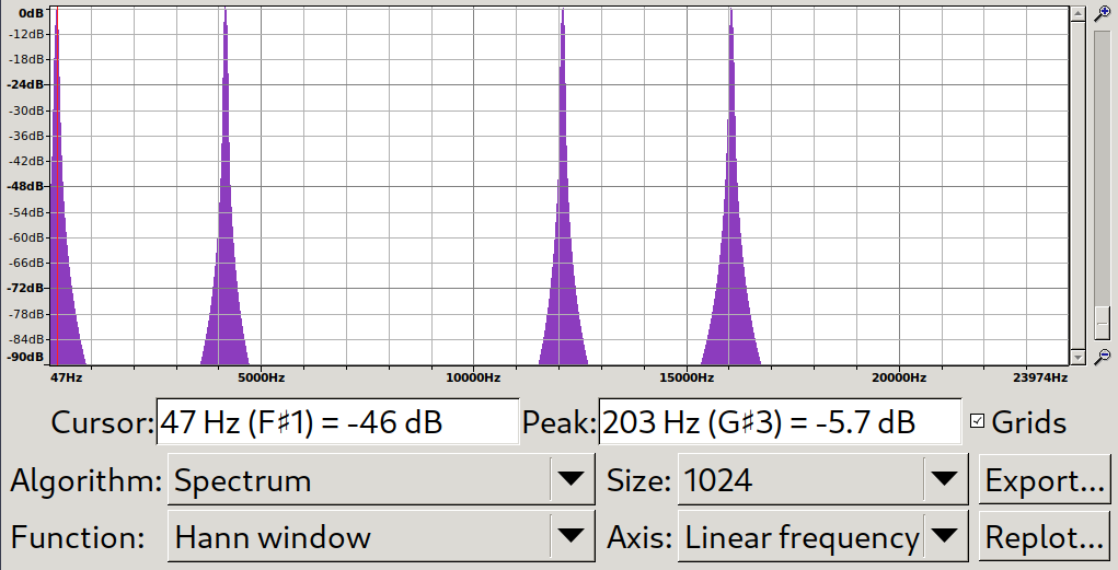
In the above screenshots, looking for instance at the first peak shows a much bigger imprecision when using the rectangular window rather than with the Hann window (the real frequency being 200 Hz).

Catching “pops” within a lengthy file

If there are defects that can be heard often in the file (like if you have some kind of repeating DMA underrun), these will be caught by the above algorithm. However, if it happens only once, if the level of the noise is not so loud compared to the signal and if the recording duration is big, we might miss it.

In order to prevent this from happening, we can perform the FFT using a sliding window. That is, instead of checking once all the samples, performing several FFTs on smaller windows evenly distributed over the recording. All frequencies should be logged, so if there is a parasitic frequency somewhere in the file, we should find it because it might become significant within a smaller window.

Final interface for frequency analysis

Analyzing *.wav files is now extremely easy, just feed the tool:

arecord | ./wav-analyzer

If the analyzed file comes from wav-generator, you can even tell the tool, so it will use the same heuristics to check the presence of the expected frequencies:

$ ./wav-generator -c2 -r48000 -d10 -f2 2>/dev/null | ./wav-analyzer -f2
Analyzing audio file with following parameters:
* Channels: 2
* Sample rate: 48000 Hz
* Bits per sample: S32_LE
* Duration: 10 seconds
* Frequencies per channel: 2

Frequencies expected on channel 0 (max threshold: 4084.3):
* 0/ 200 Hz: ok (-1 Hz)
* 1/ 12100 Hz: ok
Frequencies expected on channel 1 (max threshold: 4094.8):
* 0/ 4166 Hz: ok
* 1/ 16066 Hz: ok (-1 Hz)

The source code is available on Github, just clone it and run make from the root directory.

Can you use the tool with music files instead of destroying your ears with pure sine-waves during real-life testing? While in theory totally possible, the tool has not been designed for that, but it could definitely be improved to do something like that. The roots of the famous Shazam app are not so magic, after all!